Latent Matters
Learning Deep State-Space Models
Have you ever had difficulties training deep state-space models with variational inference?
Deep state-space models are great at modelling dynamical systems — especially if your only source of information is image data. But sometimes, no matter what we try, the model does not train properly and we get poor predictions.
In this blog post we will get to the bottom of the problem. Spoiler: the latent representation of the system is what matters — and we propose a solution on how to correctly learn it.
This work has been published at the Thirty-Fifth Conference on Neural Information Processing Systems (NeurIPS 2021).
Background: dynamical systems and how to model them
Dynamical systems
Let us first look into a well-known dynamical system that is widely used for experimental verification: the pendulum environment. The pendulum, being subject to gravity, is controlled by a one degree-of-freedom torque, the action.
Our goal is to learn a model with which we can predict this dynamical system, while the only source of information available to us is sequences of images of the moving pendulum.
To collect a dataset \(\mathcal{D}=\big\{\mathbf{x}_{1:T}^{(n)}, \mathbf{u}_{1:T}^{(n)}\big\}_{n=1}^N\), we typically observe the environment at discrete time steps. Here, \(\mathbf{x}_{1:T}=(\mathbf{x}_1, \mathbf{x}_2, \dots, \mathbf{x}_T)\) represents a sequence of images of the pendulum, and \(\mathbf{u}_{1:T}\) are the applied actions. The challenge now is to infer the dynamics of the system from the obtained data.
Deep state-space models
A powerful approach for describing dynamical systems on the basis of image data and accounting for the resulting uncertainty is deep state-space models (DSSMs).
The idea is to model the unknown distribution of observed sequence data by means of typically lower-dimensional latent variables \(\mathbf{z}_{1:T}\):
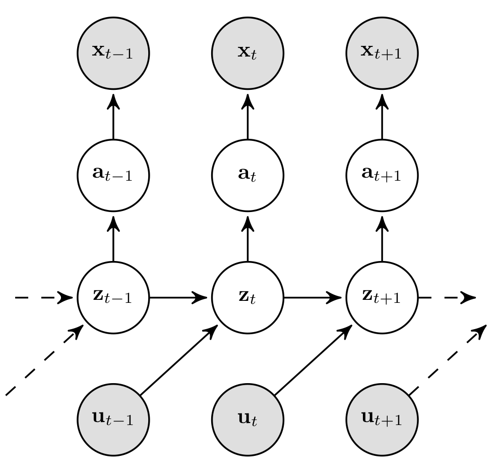
In DSSMs, latent variables are supposed to represent the underlying state of the system. In case of the pendulum, for example, the state consists of the rotation angle and the angular velocity. This is typically achieved by imposing the Markov assumption, which states that the future is independent of the past given the present. In other words: the current observation \(\mathbf{x}_t\) and the future state \(\mathbf{z}_{t+1}\) only depend on the state and action at \(t\), i.e. \(\mathbf{z}_t\) and \(\mathbf{u}_t\), as depicted by the graphical model below:
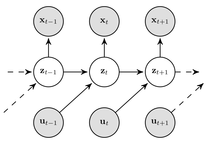
The corresponding probabilistic notation can be derived as follows:
As a consequence, the dynamics underlying the observed system are modelled by the transition model and the mapping to the observation space is achieved by the observation model. This has two major advantages: first, we learn a latent representation of the dynamical system that is interpretable since the state space reflects our understanding of physics; second, it allows us to model arbitrary long sequences with a fixed number of parameters \(\theta\).
Note: the term deep in DSSMs refers to the fact that the distributions \(p_\theta(\mathbf{x}_t\vert\,\mathbf{z}_t)\) and \(p_\theta(\mathbf{z}_t\vert\,\mathbf{z}_{t-1},\mathbf{u}_{t-1})\) are parametrised by neural networks, which allow us to learn highly nonlinear dependencies.
Learning deep state-space models with variational inference
A powerful framework for learning DSSMs is (amortised) variational inference. It is based on maximising the sequential evidence lower bound (ELBO):
where \(p_\mathcal{D}(\mathbf{x}_{1:T},\mathbf{u}_{1:T})\) is the empirical distribution representing our dataset \(\mathcal{D}\).
The idea of the ELBO is to introduce a variational distribution \(q_\phi(\mathbf{z}_{1:T}\vert\,\mathbf{x}_{1:T}, \mathbf{u}_{1:T})\) that approximates the posterior \(p_\theta(\mathbf{z}_{1:T}\vert\,\mathbf{x}_{1:T}, \mathbf{u}_{1:T})\), which is usually intractable in the context of neural models. However, we need the posterior to learn \(p_\theta(\mathbf{x}_{1:T}, \mathbf{z}_{1:T}\vert\,\mathbf{u}_{1:T})\) — and in this context, the classical expectation–maximisation algorithm reveals the beauty of the ELBO:
It can be shown that by maximising the ELBO w.r.t. \(\phi\), we optimise the variational distribution towards the posterior; and by maximising the ELBO w.r.t. \(\theta\), we approximate the classical maximum likelihood learning. However, for neural models it is standard practice to optimise the parameters \(\theta\) and \(\phi\) jointly via a stochastic gradient-based optimisation, as introduced by Kingma and Welling (2014).
Let us conclude by briefly touching on another crucial detail: the parametrisation of the approximate posterior \(q_\phi(\mathbf{z}_{1:T}\vert\,\mathbf{x}_{1:T}, \mathbf{u}_{1:T})\). There exist several approaches, and most of them rely on recurrent neural networks (RNNs). Two popular representatives are deep Kalman filters/smoothers (Krishnan et al., 2015), (Krishnan et al., 2017) and deep variational Bayes filters (Karl et al., 2017). For an introduction to the latter, we highly recommend our previous blog post.
Boosting the prediction accuracy of deep state-space models
Although variational inference is a powerful framework for learning DSSMs, it does have some weaknesses. The most significant are:
- The ELBO is prone to local optima with the consequence that the model often does not learn the correct system dynamics;
- RNNs are typically used to parametrise \(q_\phi(\mathbf{z}_{1:T}\vert\,\mathbf{x}_{1:T}, \mathbf{u}_{1:T})\), and thus to approximate classical Bayesian filtering or smoothing. However, this often results in less accurate models.
In the following sections, we will address these problems and propose solutions to them. Note that we will focus on smoothing posteriors, as these generally allow for a more accurate inference. A blog post covering this topic can be found here.
Balancing the evidence lower bound
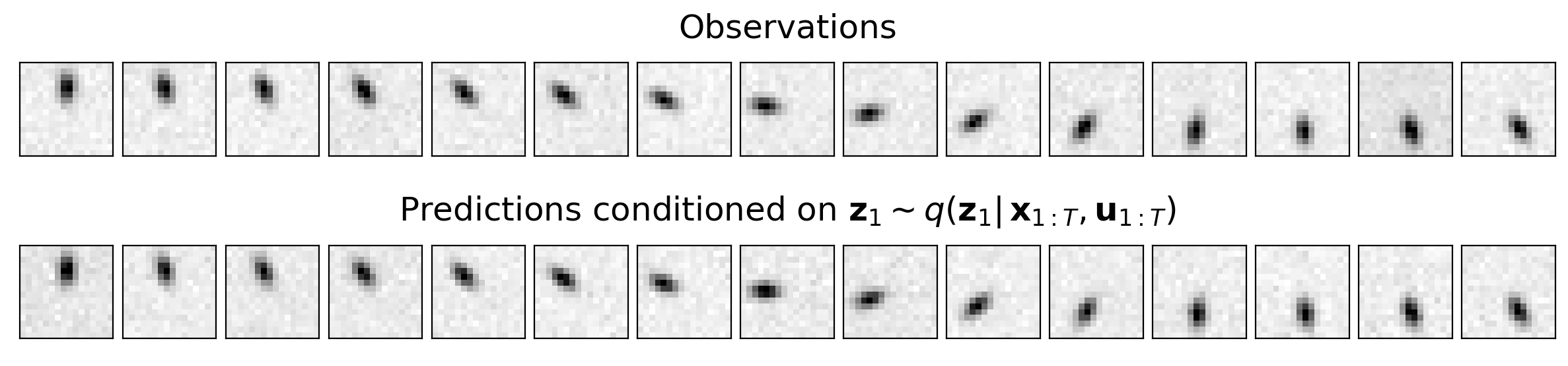
Sometimes, no matter what we try, our model is not capable of predicting the observed environment — even though we achieve high ELBO values that are comparable to the state-of-the-art on our dataset. The resulting predictions might look like this:
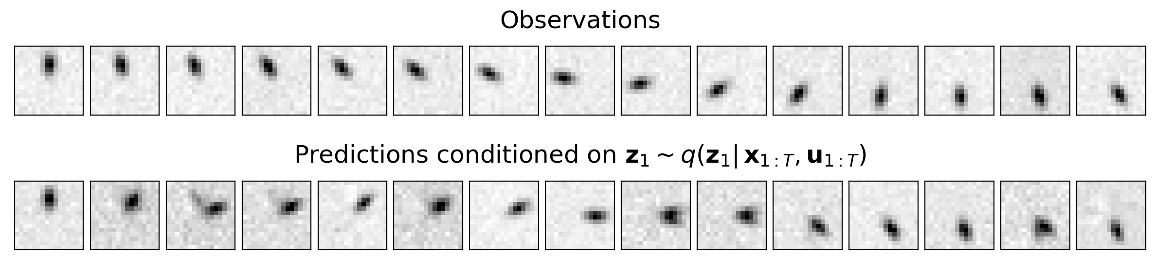
In theory, our model should predict a sequence that corresponds to the observed one. This is because we start at the same state \(\mathbf{z}_1\), which we obtain through \(q_\phi(\mathbf{z}_{1}\vert\,\mathbf{x}_{1:T}, \mathbf{u}_{1:T})\), and apply the same actions \(\mathbf{u}_{1:T}\). Thus, our transition model \(p_\theta(\mathbf{z}_t\vert\,\mathbf{z}_{t-1},\mathbf{u}_{t-1})\) should predict states that — after transferred to the observation space — match the observed sequence \(\mathbf{x}_{1:T}\). However, the transition model obviously did not learn the correct system dynamics. Note that the observation model is usually not the cause of the problem, as can be verified by the correct reconstruction \(\mathbf{x}_1\) of the smoothed initial state.
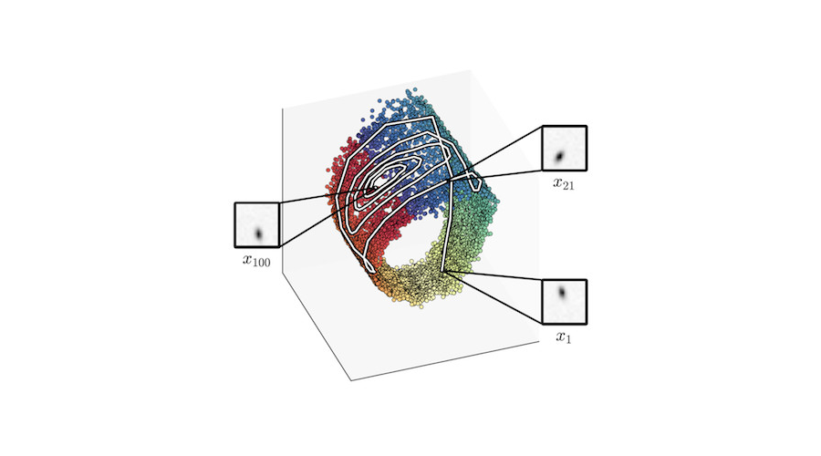
To get to the bottom of this problem, we first visualise the inferred state-space representation \(\mathop{\mathbb{E}_{p_\mathcal{D}(\mathbf{x}_{1:T},\mathbf{u}_{1:T})}} \big[q_\phi(\mathbf{z}_{1:T}\vert\,\mathbf{x}_{1:T}, \mathbf{u}_{1:T})\big]\):
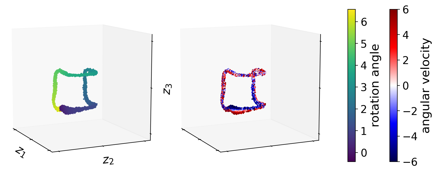
It becomes clear that the rotation angle (left plot) is properly inferred; the representation of the angular velocity (right plot), by contrast, appears messy. Despite the fact that \(p_\theta(\mathbf{z}_t\vert\,\mathbf{z}_{t-1},\mathbf{u}_{t-1})\) is parametrised by a neural network, the above representation of the angular velocity makes it significantly harder to find a general rule for mapping \(\mathbf{z}_{t-1}\) to \(\mathbf{z}_{t}\), and thus to learn an accurate transition function.
What causes local optima as in the example above? By taking into account the Markov assumption, we can divide the ELBO into the following two components:
To simplify the notation, we resort to the rate–distortion theory. Minimising the distortion \(D(\theta,\phi)\) optimises the model's ability to reconstruct observations; whereas minimising the rate \(R(\theta, \phi)\) enables the model to learn the underlying dynamics of the observed system.
If rate and distortion are not balanced during training, we can easily end up in a local optimum, as shown in the figure above. This is because different combinations of rate and distortion can result in similar ELBO values. Therefore, high ELBO values do not necessarily imply that the model has learned the correct system dynamics.
To balance distortion and rate during training, we formulate the ELBO as the Lagrangian of a constrained optimisation problem by imposing the inequality constraint \(D(\theta, \phi)\leq D_0\):
where the Lagrange multiplier \(\lambda\) can be viewed as a weighting term for the distortion, and \(D_0\) is a hyperparameter defining the baseline for our desired reconstruction quality. This approach enables us to ensure a good reconstruction quality, i.e. a low \(D(\theta, \phi)\), and thus to provide a sufficient basis for learning the underlying system dynamics.
The original EM algorithm for optimising the ELBO, which we described in the previous section, provides the following connection to the constrained optimisation problem (Klushyn et al., 2019):
Here, unlike in the original EM algorithm, we want \(q_\phi(\mathbf{z}_{1:T}\vert\,\mathbf{x}_{1:T}, \mathbf{u}_{1:T})\) to additionally satisfy the inequality constraint \(D(\theta, \phi)\leq D_0\) in the E-step. An introduction to the optimisation algorithm can be found in our previous blog post.
If we use the above Lagrangian for learning DSSMs, distortion and rate are balanced by the Lagrange multiplier \(\lambda\) allowing the system to properly infer the rotation angle and the angular velocity:

As can be seen in the figure, \(\lambda\) is updated such that the model first improves the reconstruction quality/constraint by learning the rotation angle (see epoch 70). And as soon as the constraint is satisfied, \(\lambda\) decreases and the model starts learning the underlying dynamics, i.e. to represent the angular velocity.
The above state space provides the simplest representation of our pendulum environment, and therefore forms the optimal basis for learning an accurate transition model. As shown by the predicted sequence, \(p_\theta(\mathbf{z}_t\vert\,\mathbf{z}_{t-1},\mathbf{u}_{t-1})\) has learned the correct system dynamics of the pendulum environment:
Combining variational inference with classical Bayesian smoothing
In the context of DSSMs, most variational methods use RNNs to define \(q_\phi(\mathbf{z}_{1:T}\vert\,\mathbf{x}_{1:T}, \mathbf{u}_{1:T})\). A popular approach, e.g. (Krishnan et al., 2015), is to learn the parameters of the approximate posterior by means of a bidirectional LSTM, which is expected to replace classical Bayesian smoothing.
However, as we experimentally confirm in our paper, RNN-based approaches often infer the dynamics — i.e. the mapping from \(\mathbf{z}_{t-1}\) to \(\mathbf{z}_t\) — less accurately than classical Bayesian smoothing. Although it seems conclusive that closed-form Bayesian inference is more precise, we would like to point out a further important source of inaccuracy associated with RNNs: they can be used to parametrise \(q_\phi(\mathbf{z}_{t}\vert\, \mathbf{x}_{1:T}, \mathbf{u}_{1:T})\) but not \(q_\phi(\mathbf{z}_{t}\vert\, \mathbf{z}_{t-1},\mathbf{x}_{t:T}, \mathbf{u}_{t-1:T})\). The latter, however, is necessary to correctly factorise \(q_\phi(\mathbf{z}_{1:T}\vert\,\mathbf{x}_{1:T}, \mathbf{u}_{1:T})\). Therefore, RNN-based approaches rely on restricting assumptions or require workarounds, cf. (Krishnan et al., 2015), (Krishnan et al., 2017), (Karl et al., 2017), (Karl et al., 2017).
Classical Bayesian smoothing, on the other hand, requires a linear or linearised transition and observation model. Especially in the domain of high-dimensional image data that describe nonlinear dymanics, a liniarisation can be computationally expensive and is therefore often unfeasible.
To get the best of both variational inference and classical Bayesian smoothing, we propose an novel method for learning DSSMs, which we refer to as extended Kalman VAE (EKVAE). For this purpose, we leverage the concept of extended Kalman smoothers, but avoid the expensive linearisation (Taylor expansion) of the transition and observation model.
In a first step, we evade the linearisation of \(p_\theta(\mathbf{x}_t\vert\,\mathbf{z}_t)\) by introducing auxiliary variables \(\mathbf{a}_{1:T}\):
This allows us to define a linear auxiliary observation model,
which can be used for extended Kalman smoothing instead of the original observation model \(p_\theta(\mathbf{x}_t\vert\,\mathbf{z}_t)\), as we will discuss in more detail a little later. The highly nonlinear mapping to the observation space is now realised through \(p_\theta(\mathbf{x}_t\vert\,\mathbf{a}_t)\) that we parametrise by a neural network.
In order to linearise \(p_\theta(\mathbf{z}_t\vert\,\mathbf{z}_{t-1},\mathbf{u}_{t-1})\), we use a proven approach that is particularly well suited for the lower-dimensional state space. The idea is to approximate nonlinear dynamics directly by a locally-linear transition model, e.g. (Watter et al., 2015),
which is designed to globally find the best linearisation at each time step as a function of the previous state and action. The functions \(\mathbf{F}_\theta\), \(\mathbf{B}_\theta\), and \(\mathbf{Q}_\theta\) are typically modelled by a set of learnable base matrices that are weighted by a neural network. This approach allows us to apply the extended Kalman smoother algorithm, but replace the computationally expensive Taylor expansion with \(\mathbf{F}_\theta\) and \(\mathbf{B}_\theta\).
Let us now take a closer look at how inference works in the EKVAE. The introduced auxiliary variables allow us to divide the original approximate posterior into two components, \(\prod_{t=1}^T q_\phi(\mathbf{a}_t\vert\,\mathbf{x}_t)\) and \(p_\theta(\mathbf{z}_{1:T}\vert\,\mathbf{a}_{1:T}, \mathbf{u}_{1:T})\). To illustrate this, we demonstrate the inference process on the example of the pendulum:
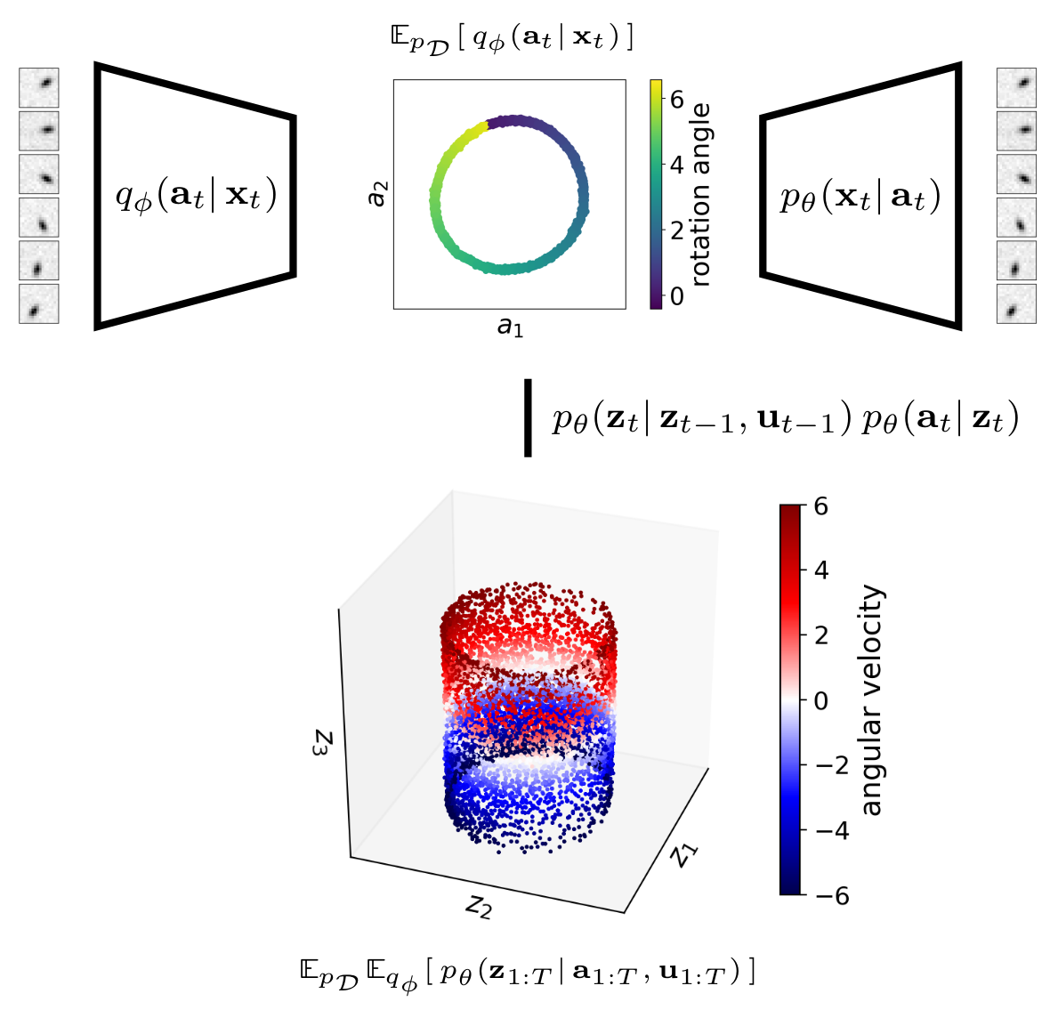
First, the observable part of the state — i.e. the rotation angle — is inferred through the encoder–decoder pair \(q_\phi(\mathbf{a}_t\vert\,\mathbf{x}_t)\) and \(p_\theta(\mathbf{x}_t\vert\,\mathbf{a}_t)\); both distributions are parametrised by neural networks. Therefore, this works similar to the classical variational autoencoder (VAE) (Kingma and Welling, 2014) and is well suited for high-dimensional image data.
Second, we use samples \(\mathbf{a}_{1:T}\) in conjuction with the locally-linear Gaussian \(p_\theta(\mathbf{z}_t\vert\,\mathbf{z}_{t-1},\mathbf{u}_{t-1})\) and the linear Gaussian \(p_\theta(\mathbf{a}_t\vert\,\mathbf{z}_t)\) to infer the full state including the dynamics — i.e. the angular velocity — via extended Kalman smoothing; that is, by computing \(p_\theta(\mathbf{z}_{1:T}\vert\,\mathbf{a}_{1:T}, \mathbf{u}_{1:T})\) in closed form.
As we verify in our paper, the combination of variational inference with classical Bayesian smoothing significantly increases the prediction accuracy of the learned model. This is because the inference of the dynamics is more accurate and we avoid the problem of parametrising \(q_\phi(\mathbf{z}_{t}\vert\, \mathbf{z}_{t-1},\mathbf{x}_{t:T}, \mathbf{u}_{t-1:T})\).
What should we have learned?
In this blog post, we have looked at how to achieve a high prediction accuracy with deep state-space models. Here, the inferred state-space representation plays a crutial role, as it lays the foundation for learning an accurate model:
- We have demonstrated the importance of balancing the evidence lower bound during training in order to avoid local optima of the inferred state-space representation. To this end, we have reformulated the evidence lower bound as the Lagrangian of a constrained optimisation problem.
- Furthermore, a precise inference of the dynamics is decisive, i.e. of the mapping from \(\mathbf{z}_{t-1}\) to \(\mathbf{z}_t\). But this is a challenging task if our only source of information is image data. We have shown how combining variational inference with classical Bayesian smoothing addresses this problem.
Deep latent-variable models are often treated as black boxes. The bottom line of this blog post is that we should take a closer look at the learned latent representation of our data. Especially, in the context of deep state-space models, this can provide the decisive clue to identify our problem.
For a more detailed discussion and an extensive experimental evaluation, we refer to our paper (Klushyn et al., 2021).
Bibliography
Maximilian Karl, Maximilian Soelch, Justin Bayer, and Patrick van der Smagt. Deep variational Bayes filters: unsupervised learning of state space models from raw data. In International Conference on Learning Representations. 2017. URL: https://arxiv.org/abs/1605.06432. ↩ 1 2
Maximilian Karl, Maximilian Soelch, Philip Becker-Ehmck, Djalel Benbouzid, Patrick van der Smagt, and Justin Bayer. Unsupervised Real-Time Control through Variational Empowerment. In International Symposium on Robotics Research (ISRR). 2017. URL: https://arxiv.org/abs/1710.05101. ↩
Diederik P. Kingma and Max Welling. Auto-encoding variational Bayes. In International Conference on Learning Representations. 2014. ↩ 1 2
Alexej Klushyn, Nutan Chen, Richard Kurle, Botond Cseke, and Patrick van der Smagt. Learning Hierarchical Priors in VAEs. In Advances in Neural Information Processing Systems. 2019. URL: https://arxiv.org/abs/1905.04982. ↩
Alexej Klushyn, Richard Kurle, Maximilian Soelch, Botond Cseke, and Patrick van der Smagt. Latent Matters: Learning Deep-State-Space Models. In Advances in Neural Information Processing Systems. 2021. URL: https://openreview.net/forum?id=-WEryOMRpZU. ↩
Rahul G. Krishnan, Uri Shalit, and David Sontag. Deep Kalman Filters. arXiv preprint arXiv:1511.05121, 2015. ↩ 1 2 3
Rahul G. Krishnan, Uri Shalit, and David Sontag. Structured Inference Networks for Nonlinear State Space Models. In AAAI Conference on Artificial Intelligence. 2017. ↩ 1 2
Manuel Watter, Jost Springenberg, Joschka Boedecker, and Martin Riedmiller. Embed to Control: A Locally Linear Latent Dynamics Model for Control from Raw Images. In Advances in Neural Information Processing Systems. 2015. ↩