Less Suboptimal Learning and Control in Variational POMPDs
How to fix model-based RL by doing the obvious.
Partially-Observable Markov Decision Processes (POMDPs) are central to creating autonomous systems. Most of the interesting things we do on a daily basis are POMDPs. Humans have to make decisions with incomplete knowledge all the time. Cooking is a POMDP, since the cook has to taste the food every once in a while to make sure it is going in the right direction. Searching for the bathroom in a new building is a POMDP. A job interview is a POMDP. Shooting a basketball is a POMDP. Getting up to go to the bathroom at night is a POMDP. All two-player games that are any fun are POMDPs. We can make the list longer, but the point is that we'll have a hard time getting away from POMDPs if we ever want to do anything interesting with reinforcement learning.
Luckily, we have just the thing to address partially-observable settings: state-space models.
Deep variational state-space models (we'll call them VSSMs from now on) are a perfect fit for POMDPs. These models, by design, assume that we are observing data from a system governed by a hidden state. They are general purpose, meaning that they don't encode any inductive biases about a particular system but rather adapt to the system they are observing. Most importantly, they find a probability distribution over the system state.
VSSM-based control in POMDPs is not new. For instance, Dreamer by Hafner et al. (2021) demonstrates excellent results on challenging MuJoCo environments from pixels. MELD by Zhao et al. (2021) uses this machinery to do meta-RL. Learning to fly by BeckerEhmck et al. (2020) uses VSSMs to, well, learn to fly real drones from scratch using sensory data only. Yet despite their incredible success, the architectures used in these works contain a common, suboptimal, modelling decision: they don't inform the latent state of future observations when approximating the posterior distribution over system states given all observations. In this blog post we will focus on this decision, explain why it is suboptimal and why the benchmarks used in contemporary research might not suffer from it. We will also demonstrate how this problem becomes quite visible as one considers different benchmarks.
How PO are POMDPS?
Today's POMDP-directed research focuses on robotic environments observed with a camera. These benchmarks are quite tough in two ways:
- the observations are embedded in high-dimensional images;
- the system dynamics are often complex.
The performance that Dreamer achieves on a system that is as complex as Humanoid, based on images only, is impressive. But is Humanoid a tough benchmark in terms of partial observability? In the appendix of (Srinivas et al., 2020) a very interesting experiment can be found. By doing regression on the robot state based on a shallow stack of video frames, they show that system identification is easily achievable in MuJoCo just by looking at the recent past. On an intuitive level, this speaks against the MuJoCo-benchmarks being a good measure of how good VSSMs are at solving POMDPs.
Taking a closer look at many of the most successful papers on POMDPs, we see an emphasis more on representation learning, i.e., modelling the environment, rather than state estimation (i.e., knowing where I am in that environment). While representation learning is undoubtedly important, it does not bring us all the way to the finish line. POMDPs, as opposed to MDPs, used to be much more about maintaining a belief over the system state and trading off between reducing one's uncertainty and reducing future cost.
Looking at earlier work on POMDPs, we see researchers focusing on simple problems designed to force agents to actively seek out missing information. The Heaven and Hell benchmark is a great example. Let's review it and see how it differs from the current image-based MuJoCo benchmarks.
Heaven and Hell
The Heaven and Hell problem was introduced in (Thrun, 1999). It features a room with four walls. The agent is in the lower-left corner and it must either reach the upper-left or the lower-right corner. The agent does not know which corner the agent has to reach in a given episode until it visits the upper-right corner, where it receives that information from what is called a priest. The problem is confounded by the fact that the agent cannot observe its location, and can only sense its environment by bumping into one of the walls, at which point it is told which wall it hit. On top of this, some random noise is injected into the agent's movements. A successful agent in Heaven and Hell has to learn to navigate to the opposite corner from where it started (where the priest is) and then proceed to whichever corner it is told to be Heaven. Since there is noise, the agent cannot rely on an open-loop policy for finding the priest.
What is so striking about Heaven and Hell as a POMDP is that it features two different types of partial observability. First, the agent does not know its own location and it does not know the noise that will perturb its desired motion. Therefore, it has to learn to estimate its location by touching walls. Second, the agent cannot directly start reducing its cost, but has to first learn the location of Heaven. Thus, Heaven and Hell requires an agent to actively make decisions to both estimate its own state, and the state of the world. By contrast, the MuJoCo benchmark only features a single type of partial observability, which is the state estimation problem where one has to estimate the robot state based on a video feed. Further, this state estimation problem cannot be made harder or easier based on the agent's behaviour, unlike Heaven and Hell, where bumping into walls makes state estimation easier, and staying away from them for long makes it harder.
Suboptimal models that work very well
Now, keeping in mind the differences between the kind of uncertainty that is introduced by looking at a system through images and the kind of uncertainty that we just described, let's review how we are addressing POMDPs with VSSMs. The structure of a POMDP and that of a state-space model closely resemble each other. In both cases we have a sequence of latent states \(\mathbf{z}_{1:T} = (\mathbf{z}_1, \mathbf{z}_2, \dots, \mathbf{z}_T)\), which give rise to observations \(\mathbf{x}_{1:T} = (\mathbf{x}_1, \mathbf{x}_2, \dots, \mathbf{x}_T)\). The system typically also contains some auxiliary values which we summarise as \(\mathbf{u}_{1:T-1}=(\mathbf{u}_{1}, \mathbf{u}_2, \dots, \mathbf{u}_{T-1})\). For our purposes, these will be the controls that are executed by the agent. For a POMDP, the observations are partitioned into regular observations and costs \(\mathbf{x}_t = [\mathbf{o}_t, \mathbf{c}_t]\). The joint distribution over observations and latent states is given by:
In deep VSSMs, we model the three distributions \(p(\mathbf{z}_1)\), \(p(\mathbf{z}_{t+1}\mid\mathbf{z}_t,\mathbf{u}_t)\), and \(p(\mathbf{x}_t\mid\mathbf{z}_t)\) with neural networks, trained by optimising the evidence lower bound (ELBO):
The ELBO depends on a fourth distribution \(q\), the approximate posterior, which is modelled using yet another neural network. The ELBO is equal to the log-likelihood \(\log p(\mathbf{x}_{1:T})\) if and only if the approximate posterior \(q\) equals the true posterior \(p(\mathbf{z}_{1:T} \mid \mathbf{x}_{1:T},\mathbf{u}_{1:T-1})\); otherwise it is a lower bound of the log-likelihood. The optimal approximate posterior is therefore the true posterior, and so it makes sense to allow this neural network to look at all of the quantities that the true posterior depends on. Yet, a trend we observe in many papers is to model \(q\) using a neural network that only looks at the current observation \(\mathbf{x}_t\) or current and past observations \(\mathbf{x}_{1:t}\). In the case of POMDPs, we even see many cases where the recognition network only looks at the regular observations \(\mathbf{o}\) and not the costs \(\mathbf{c}\).
That's often a mistake.
We believe that these modelling decisions are made for the sake of practicality. Often, we are interested in learning policies directly in latent space. This has the benefit that we do not have to render high-dimensional observations while training the policy and also eliminates the state-estimation problem from the point of view of the policy – effectively reducing the problem to an MDP (Markov Decision Process) from its perspective. These advantages are, however, complicated by the need to map observations into latent space during execution. Since the VSSM training already includes a recognition network that does exactly this, it would make sense to re-use it for that purpose. However, it is not easy to do so with a recognition network that also looks at future observations and costs, since these are not available at execution. Therefore, reducing the inputs to the recognition network to just past and present raw observations is a compromise that trades off posterior approximation for the ability to reuse the recognition network as a filter at execution and train the policy entirely in latent space. Naturally, the question now is how dangerous it is to make that tradeoff, which is exactly what our recent paper, Mind the Gap When Conditioning Amortised Inference in Sequential Latent-Variable Models (Bayer et al., 2021) deals with. In the next section, we will review its key results.
Mind the gap
In "Mind the gap", Justin Bayer, Maximilian Soelch and others focus on situations where a neural approximate posterior distribution \(q\) is not given access to all of the quantities that the respective true posterior depends on. Formally, if we partition the conditions of the true posterior \(\mathbf{z} \mid \tilde C\) into two sets \(\tilde C := [C, \bar C]\), where the approximate posterior only considers \(C\) and not \(\bar C\), then the following statements are true:
- The ELBO-optimal neural approximate posterior matches neither \(p(z \mid C)\) nor \(p(z \mid C, \bar C)\),
- The ELBO-optimal generative model under the optimal neural approximate posterior does not match the maximum-likelihood model,
unless \(p(\mathbf{z} \mid C) = p(\mathbf{z} \mid C, \bar C)\). This last condition would imply that the future holds no information about the present when one considers the past and the present. Bayer et al. call this phenomenon the conditioning gap. For VSSM-based learning with POMDPs, \(\mathbf{z}\) is \(\mathbf{z}_t\), and the sets \(C\) and \(\bar C\) can defined in different ways. In the typical case, \(C := \mathbf{o}_{1:t}\) and \(\bar C := (\mathbf{o}_{t+1:T}, \mathbf{c}_{1:T})\). What the conditioning gap tells us for POMDPs is that, unless we are in a system where costs and future observations give us no additional information about the hidden state after observing past and present observations, we run the risk of learning a biased generative model by using a recognition network that doesn't look at costs and future observations.
More details in this blog entry.
Now, it is perhaps surprising that many recent works seem to take that risk, while still being able to solve their tasks. We believe that this is due to differences between past and present POMDP benchmarks, as discussed above. As we move to systems with higher levels of partial-observability, we expect to see the conditioning gap taking effect.
How do we check this?
It's easy to devise a way of checking how big a problem all this is for model-based reinforcement learning (MBRL): construct the same MBRL pipeline twice, the only difference between the two being the recognition network used to train the VSSM. In one case we use an RNN that goes forward in time; in the other, a bidirectional RNN. The policy is a recurrent network trained on observations generated by the VSSM. Crucially this means that between the two setups, the only difference is the recognition network used during training the VSSM. Everything before and after that point is the same. Both pipelines use a recurrent policy to gather data and both train that policy by using the transition and emission models of the VSSM. Our hypothesis: systems with strong partial observability will suffer from the conditioning gap when training the VSSM and will have to work with biased generative models, leading to suboptimal policies.
Simple problems for simple hypotheses
In the spirit of Heaven and Hell, we'd like to test our hypothesis on simple, continuous problems. We'd also ideally like to see how the conditioning gap behaves under different kind of partial observability. On the "very-hard-to-observe"-end of the spectrum, we have an environment called Dark Room, featuring an agent trapped in a pitch-black room with 4 walls. The agent wants to go to the centre of the room but does not know where it is. It has to first find a wall by bumping into it and then follow it to a corner, after which it can reach the centre easily. To solve this environment, the agent has to actively make decisions that reduce its uncertainty about its location before trying to reduce the actual cost (which is 0 at the centre and 1 everywhere else). We implement the simplest possible version of this task as a 2D environment.
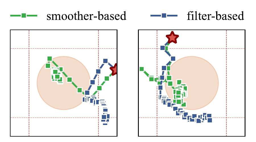
The Mountain Hike environment (Igl et al., 2018) is another 2D problem where a point-agent needs to reach a certain location. In this case, the agent's life is made harder by a peculiarly-shaped cost landscape, where straying from a corridor of safety leads to increased cost. Mountain Hike is a POMDP through two restrictions. First, the agent is only able to observe its location with some additive noise. Second, the transition function adds some random unobserved noise to the location of the agent. Mountain Hike is in some sense the simplest kind of partially-observable system: one in which we can observe the true system through some white noise.
Finally, we consider a meta-learning-like scenario by putting a simple twist to the most common control problem of all. We take a pendulum but set its mass at random at the beginning of an episode.
On these three environments, we want to assess the effect of the conditioning gap on MBRL.
Comparing populations of experiments
RL algorithms are notoriously hard to compare. Many papers compare best-possible hyperparameter configurations for different methods based on a small number of random seeds.
We take a different approach. For each pipeline, we do a hyperparameter search over different values such as the number of layers of the transition network or the batch size used to train the policy. Then, for each such hyperparameter search we identify a cluster of experiments – each being a single run of the algorithm with said hyperparameters – that "solve" the corresponding task. Finally, we compare all experiments that solve the task for the filter with those of the smoother. This way, we want the illustrate the effect of the conditioning gap across hyperparameters and in a general sense. We base our comparison on regret, which is the difference in cost to executing an optimal policy. (Since our environments are relatively simple we can implement them using the autodiff framework JAX. This allows obtaining a near-optimal policy by training with gradient descent on the true system.)
Results
If we compare populations of best-performing hyper-parameter configurations, we get the following:
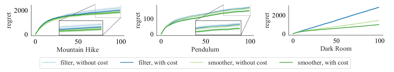
These are regret curves we are looking at. The regret curve of an optimal agent would just be a flat line at zero. A learning agent generally cannot have such a regret curve, though successful learning agents have saturating regret curves, indicating that the learner eventually reaches an optimal policy.
Let's start by looking at Mountain Hike, arguably the closest of the three to being fully observable. Here, smoothers are not dramatically better than filters: both models obtain saturating regret curves. Still, smoothers represent an upper bound on the performance of filters in average. This is what we would expect – on a well-observable problem, the average smoother should be "greater than or equal to" the average filter. Moving on to the pendulum with randomly sampled mass, which contains an interesting state estimation problem, we see the gap starting to widen. The difference is still not so large that we can see it without zooming in, though it is there. Finally, as we reach Dark Room, the least observable of the three, we see that filters are absolutely incapable of coping with the missing information. The difference between filters and smoothers is not incremental here. The filter is stuck with a linear regret curve, indicating that the optimal policy is never found. One class of models has saturating regret as the other does not, even though the only difference between the two is a seemingly innocuous modelling decision in the recognition network, one that many code bases capable of producing great results have made.
Outlook
Our work, of course, is not done. If anything, the vast difference between Dark Room and Mountain Hike reveals that we need to carefully consider different types of partial observability. We can envision problems where information is missing due to the presence of other agents whose intrinsics we are not privy to. The simple constant noise of Mountain Hike might be replaced by a noise model that depends on the actions of the agent, e.g., a motion sensor that is less accurate at certain velocities. Ultimately, we wish to reach a taxonomy of partial observability that allows us to come up with simple principles that guide modeling decisions; being able to say "this problem only has some simple constant noise, therefore omitting the future inputs might be acceptable", or "this problem would probably exhibit a large conditioning gap, therefore we need to use a BiRNN".
For a more detailed version of this blog post, you can check out our paper Less Suboptimal Learning and Control in Variational POMDPs, which was part of the Self-Supervision for Reinforcement Learning workshop at ICLR 2021. We also highly encourage you to have a look at the original paper on the conditioning gap, Mind the Gap When Conditioning Amortised Inference in Sequential Latent-Variable Models, which was presented at the main conference of the same year. Maximilian Soelch has written a wonderful blog post on the subject, here at argmax.
Bibliography
Justin Bayer, Maximilian Soelch, Atanas Mirchev, Baris Kayalibay, and Patrick van der Smagt. Mind the gap when conditioning amortised inference in sequential latent-variable models. In International Conference on Learning Representations. 2021. URL: https://openreview.net/forum?id=a2gqxKDvYys. ↩
Philip Becker-Ehmck, Maximilian Karl, Jan Peters, and Patrick van der Smagt. Learning to fly via deep model-based reinforcement learning. 2020. URL: https://arxiv.org/abs/2003.08876, arXiv:2003.08876. ↩
Danijar Hafner, Timothy Lillicrap, Mohammad Norouzi, and Jimmy Ba. Mastering atari with discrete world models. 2021. arXiv:2010.02193. ↩
Maximilian Igl, Luisa M. Zintgraf, Tuan Anh Le, Frank Wood, and Shimon Whiteson. Deep variational reinforcement learning for pomdps. In Jennifer G. Dy and Andreas Krause, editors, Proceedings of the 35th International Conference on Machine Learning, ICML 2018, Stockholmsmässan, Stockholm, Sweden, July 10-15, 2018, volume 80 of Proceedings of Machine Learning Research, 2122–2131. PMLR, 2018. URL: http://proceedings.mlr.press/v80/igl18a.html. ↩
Aravind Srinivas, Michael Laskin, and Pieter Abbeel. CURL: contrastive unsupervised representations for reinforcement learning. 2020. arXiv:2004.04136. ↩
Sebastian Thrun. Monte carlo pomdps. In Proceedings of the 12th International Conference on Neural Information Processing Systems, NIPS'99, 1064–1070. Cambridge, MA, USA, 1999. MIT Press. ↩
Tony Z. Zhao, Anusha Nagabandi, Kate Rakelly, Chelsea Finn, and Sergey Levine. Meld: meta-reinforcement learning from images via latent state models. 2021. arXiv:2010.13957. ↩